Metric spaces of microbial essential gene landscapes
Published:
Essential genes are those which are crucial for survival of an organism in a given context. This post will introduce manifold and metric learning to characterize and classify essential genes from the chaos game representation of a genetic sequence.
This post will be an instructional guide to constructing metric spaces and perform manifold learning in Python.
Briefly, what are metric spaces?
A metric space, without too much mathematical abstraction, is just a set of data points together with a concept of distance between the data points. The distance between points is given as the output of a function and this function is typically called the metric. To reveal a bit of what’s to come, we are wanting to identify a metric space in which essential genes and non-essential genes are distant from each other. Right now, it is unclear what the space looks like and what the right metric is. Let’s see if we can find a metric space with our desired properties.
Learning essential gene landscapes
import collections
from collections import OrderedDict
from matplotlib import pyplot as plt
from matplotlib import cm
import seaborn as sns
import numpy as np
import pandas as pd
pd.options.mode.chained_assignment = None
from Bio import SeqIO # biopython used for parsing fasta files of sequences
import gzip # to read the compre
import scanpy as sc
plt.style.use('dark_background')
plt.rcParams.update({'font.size':22});
plt.rcParams.update({'axes.linewidth':1.5})
The database of essential genes
This is a database compiled by researchers at Tianjin University and includes essential gene sequence and annotations from roughly 100 organisms spanning bacteria, archaea, and eukaryotes. You can find the database of essential genes here.
In this post, we will focus on the analysis of bacterial essential gene sequences. You can download the annotations and nucleic acid sequences from here. The filename for the bacteria annotations is deg_annotation_p.csv and for the essential gene nucleic acid sequences is DEG10.nt.gz. This sequence file is in fasta format and we will go over how to parse such files with biopython
Let’s start by reading in the annotations. We’ll use pandas
anno_df = pd.read_csv('deg_annotation_p.csv', sep=';', header=None,quotechar='"')
anno_df.head(2)
| 0 | 1 | 2 | 3 | 4 | 5 | 6 | 7 | 8 | 9 | 10 | 11 | 12 | 13 | |
|---|---|---|---|---|---|---|---|---|---|---|---|---|---|---|
| 0 | DEG1001 | DEG10010001 | dnaA | 16077069 | COG0593L | DNA replication | initiation of chromosome replication | Bacillus subtilis 168 | NC_000964 | Rich medium | - | GO:0005737 GO:0005524 GO:0003688 GO:0006270 GO... | P05648 | NaN |
| 1 | DEG1001 | DEG10010002 | dnaN | 16077070 | COG0592L | DNA replication | DNA polymerase III (beta subunit) | Bacillus subtilis 168 | NC_000964 | Rich medium | - | GO:0005737 GO:0009360 GO:0008408 GO:0003677 GO... | P05649 | NaN |
The annotations are missing column names. Let’s assign names to most of the columns
anno_df.columns = ['organism_id','gene_id','gene','protein_id?','?','biological process',
                   'biological function','bacteria','genome_ref','media','locus_tag','GO_id','??','???']
anno_df.head(2)
| organism_id | gene_id | gene | protein_id? | ? | biological process | biological function | bacteria | genome_ref | media | locus_tag | GO_id | ?? | ??? | |
|---|---|---|---|---|---|---|---|---|---|---|---|---|---|---|
| 0 | DEG1001 | DEG10010001 | dnaA | 16077069 | COG0593L | DNA replication | initiation of chromosome replication | Bacillus subtilis 168 | NC_000964 | Rich medium | - | GO:0005737 GO:0005524 GO:0003688 GO:0006270 GO... | P05648 | NaN |
| 1 | DEG1001 | DEG10010002 | dnaN | 16077070 | COG0592L | DNA replication | DNA polymerase III (beta subunit) | Bacillus subtilis 168 | NC_000964 | Rich medium | - | GO:0005737 GO:0009360 GO:0008408 GO:0003677 GO... | P05649 | NaN |
We see that each gene has a gene_id and corresponding organism_id. Keep in mind that not every gene has a name and so gene_id will be used as the unique identifier. Also, as we will see in the sequence fasta file, the gene_id is used as the ID and Name of a sequence
How many unique bacteria are there in the database?
len(anno_df['bacteria'].unique())
82
Next let’s take a look at the sequence file and print a record for a single sequence
with gzip.open("DEG10.nt.gz", "rt") as handle:
    for record in SeqIO.parse(handle, "fasta"):
        print(record)
        break
print(type(record.seq))
ID: DEG10010001
Name: DEG10010001
Description: DEG10010001
Number of features: 0
Seq('ATGGAAAATATATTAGACCTGTGGAACCAAGCCCTTGCTCAAATCGAAAAAAAG...TAG')
<class 'Bio.Seq.Seq'>
We can see that the sequence is stored in record.seq as a Bio.Seq.Seq object. This can be converted to a string object
str(record.seq)
'ATGGAAAATATATTAGACCTGTGGAACCAAGCCCTTGCTCAAATCGAAAAAAAGTTGAGCAAACCGAGTTTTGAGACTTGGATGAAGTCAACCAAAGCCCACTCACTGCAAGGCGATACATTAACAATCACGGCTCCCAATGAATTTGCCAGAGACTGGCTGGAGTCCAGATACTTGCATCTGATTGCAGATACTATATATGAATTAACCGGGGAAGAATTGAGCATTAAGTTTGTCATTCCTCAAAATCAAGATGTTGAGGACTTTATGCCGAAACCGCAAGTCAAAAAAGCGGTCAAAGAAGATACATCTGATTTTCCTCAAAATATGCTCAATCCAAAATATACTTTTGATACTTTTGTCATCGGATCTGGAAACCGATTTGCACATGCTGCTTCCCTCGCAGTAGCGGAAGCGCCCGCGAAAGCTTACAACCCTTTATTTATCTATGGGGGCGTCGGCTTAGGGAAAACACACTTAATGCATGCGATCGGCCATTATGTAATAGATCATAATCCTTCTGCCAAAGTGGTTTATCTGTCTTCTGAGAAATTTACAAACGAATTCATCAACTCTATCCGAGATAATAAAGCCGTCGACTTCCGCAATCGCTATCGAAATGTTGATGTGCTTTTGATAGATGATATTCAATTTTTAGCGGGGAAAGAACAAACCCAGGAAGAATTTTTCCATACATTTAACACATTACACGAAGAAAGCAAACAAATCGTCATTTCAAGTGACCGGCCGCCAAAGGAAATTCCGACACTTGAAGACAGATTGCGCTCACGTTTTGAATGGGGACTTATTACAGATATCACACCGCCTGATCTAGAAACGAGAATTGCAATTTTAAGAAAAAAGGCCAAAGCAGAGGGCCTCGATATTCCGAACGAGGTTATGCTTTACATCGCGAATCAAATCGACAGCAATATTCGGGAACTCGAAGGAGCATTAATCAGAGTTGTCGCTTATTCATCTTTAATTAATAAAGATATTAATGCTGATCTGGCCGCTGAGGCGTTGAAAGATATTATTCCTTCCTCAAAACCGAAAGTCATTACGATAAAAGAAATTCAGAGGGTAGTAGGCCAGCAATTTAATATTAAACTCGAGGATTTCAAAGCAAAAAAACGGACAAAGTCAGTAGCTTTTCCGCGTCAAATCGCCATGTACTTATCAAGGGAAATGACTGATTCCTCTCTTCCTAAAATCGGTGAAGAGTTTGGAGGACGTGATCATACGACCGTTATTCATGCGCATGAAAAAATTTCAAAACTGCTGGCAGATGATGAACAGCTTCAGCAGCATGTAAAAGAAATTAAAGAACAGCTTAAATAG'
Let’s make a seq column in our annotation dataframe and append the gene sequences there
anno_df['seq'] = '' # initialize with empty string in each row
anno_df.index = anno_df['gene_id'] # set index of df to be gene_id
with gzip.open("DEG10.nt.gz", "rt") as handle:
    for record in SeqIO.parse(handle, "fasta"):
        anno_df.loc[record.id,'seq'] = str(record.seq)
Let’s also create a dataframe that contains essential gene data of a single organism. We’ll pick A. baylyi ADP1 since it is a model organism for understanding of microbiology and synthetic biology.
bacteria_df = anno_df.loc[anno_df.bacteria.isin(['Acinetobacter baylyi ADP1'])]
bacteria_df['is_essential'] = np.ones(len(bacteria_df)) # make a column noting that these genes are essential. we'll use this for modeling purposes
f'num essential genes of ADP1: {len(bacteria_df)}'
'num essential genes of ADP1: 499'
Since we want to learn the essential gene landscape (i.e. for any new gene sequence, we want to classify if the gene is essential or not by where it lies in some space that we create/learn from data), we’ll also need to know the nonessential gene sequences. Below is a function to parse the cds_from_genomic fasta file for ADP1 obtained from NCBI. This file contains gene sequences for all known protein coding genes. We will make a dataframe of all genes and note whether it is essential or not
def getRecords(fasta_sequences,essential_genes_or_tags):
    '''
    output dataframe that stores information from fasta_sequences e.g. gene_id, locus_tag, ...
    '''
    genes, locus_tags, is_essential, seqs = [],[],[],[]
    for rec in fasta_sequences:
        seqs.append(str(rec.seq))
        rec_elems = [x.strip().strip(']') for x in rec.description.split(' [')]
        if 'gene=' in str(rec_elems): # sequence has gene name (e.g. gene=dnaA)
            genes.append(rec_elems[1][5:])
            locus_tags.append(rec_elems[2][10:])
        elif 'gene=' not in str(rec_elems): # sequence has no gene name, but has locus tag
            genes.append('N/A')
            locus_tags.append(rec_elems[1][10:])
        if genes[-1] in essential_genes_or_tags or locus_tags[-1] in essential_genes_or_tags:
            is_essential.append(1)
        else:
            is_essential.append(0)

    return pd.DataFrame({'gene_id':genes,'locus_tag':locus_tags,'is_essential':is_essential,'seq':seqs})
adp1_cds_from_genomic = SeqIO.parse(open('GCA_000046845.1_ASM4684v1_cds_from_genomic.fna'),'fasta')
adp1_df = getRecords(adp1_cds_from_genomic, np.array(bacteria_df.gene)) # all adp1 cds
for column in bacteria_df.columns: # give adp1_df the same columns as bacteria_df
    if column not in adp1_df.columns:
        adp1_df[column] = ''
We can now concatenate the essential and nonessential gene rows and form our entire ADP1 essential gene dataset
adp1_df = pd.concat( ( bacteria_df, adp1_df[adp1_df['is_essential'].isin([0])] ), axis=0).reset_index(drop=True)
We now need a way to perform computations with the gene sequences. We need a gene sequence string -> unique vector function. For this task we will explore chaos game representations (CGR) as a gene sequence embedding approach and ask the questions:
Do CGRs allow us to distinguish between essential and nonessential genes? (Unsupervised approach)
If not, can we use CGRs as a starting point to learn a more meaningful representation of essential gene landscapes? (Supervised approach)
Chaos game representation
To start, I encourage you to check out the paper that first applied CGR to encode gene sequences, finding global and local structure, similarity of gene sequences, and frequency of k-mers. Briefly, the chaos game representation is formed by setting up a discrete-time dynamical system that computes the vector embedding of a gene sequence. The dynamical system has been shown to be chaotic, i.e. initial conditions that are infinitesimally close eventually become exponentially far as the system is evolved. Why this is a useful property? Well it implies that for any two gene sequences, we are likely to end up with unique vector embeddings using the chaos game representation. Below is a class which takes a sequence and length of desired k-mers and outputs the chaos game representation:
class CGR_SeqAlignment:

    def count_kmers(self, seq, k):
        '''
        Count the frequency of each k-mer in a sequence where k is an input parameter
        Inputs
        ------
            k : int
              length of each k-mer
        Returns
        -------
            kmer_dict :

        '''
        kmer_dict = collections.defaultdict(int)
        for ii in range(len(seq)-(k-1)):
            kmer_dict[seq[ii:ii+k]] +=1 # store each k-mer and its count in the seq
        for key in list(kmer_dict):   # remove any N nucleotides
            if "N" in key:
                del kmer_dict[key]
        return kmer_dict

    def get_frequencies(self, kmer_count, k):
        frequencies = collections.defaultdict(float)
        N = len(kmer_count)
        for key, value in kmer_count.items():
            frequencies[key] = float(value) / N  # probablities for each k-mer in the dict
        return frequencies

    def chaos_game_representation(self, frequencies, k):
        cgr_dim = int(np.sqrt(4**k))  # FCGR matrix size
        cgr_mat = np.zeros((cgr_dim,cgr_dim)) # chaos game representation matrix initialization

        maxx, maxy = cgr_dim, cgr_dim
        posx, posy = 0, 0
        for key, value in frequencies.items(): # finding the grids to which the k-mers belong
            for char in key:
                if char == "T":
                    posx += maxx // 2
                elif char == "C":
                    posy += maxy // 2
                elif char == "G":
                    posx += maxx // 2
                    posy += maxy // 2
                maxx = maxx // 2
                maxy = maxy//2
            cgr_mat[posy,posx] = value
            maxx = cgr_dim
            maxy = cgr_dim
            posx = 0
            posy = 0

        return cgr_mat
Let’s apply CGR to the ADP1 sequences we compiled in adp1_df
k = 4 # each CGR will have length 4^k
X = np.zeros((adp1_df.shape[0],(2**k)*(2**k))) #
cgr = CGR_SeqAlignment()
for ii, this_id in enumerate(adp1_df.index):
    seq = adp1_df.loc[this_id,'seq']
    cgr_kmers = cgr.count_kmers(seq,k)
    cgr_freq = cgr.get_frequencies(cgr_kmers,k)
    cgr_mat = cgr.chaos_game_representation(cgr_freq,k)
    cgr_mat = np.reshape(cgr_mat,(cgr_mat.shape[0]*cgr_mat.shape[1],1)) # am I convinced reshaping is done properly?
    X[ii] = np.squeeze(cgr_mat)
X contains the CGR for each gene sequence along the rows. Let’s plot the CGR for a few of these sequences.
def plot_CGR(seq,k):
    cgr = CGR_SeqAlignment()
    cgr_kmers = cgr.count_kmers(seq,k)
    cgr_prob = cgr.get_frequencies(cgr_kmers, k)
    plt.figure(); plt.title(f'CGR of a {k}-mer')
    plt.imshow(cgr.chaos_game_representation(cgr_prob, k),cmap='viridis')
    plt.gca().invert_yaxis(); plt.colorbar()
    plt.show()
plot_CGR(adp1_df.iloc[0]['seq'],k)
plot_CGR(adp1_df.iloc[-1]['seq'],k)
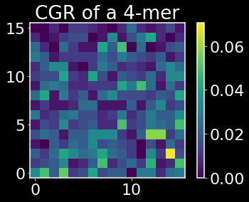
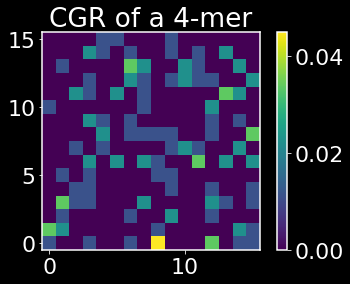
The above heatmaps show the CGRs for an essential and nonessential gene respectively. The origin corresponds to the base pair A, the lower right corner is T, the upper right is G, and the upper left is C. One useful property that can be read off from the CGRs is that if we see sparse quadrant, say e.g. the first quadrant, we can deduce that there are few k-mers that contain in that sequence that contain a T followed by a G or a C followed by a G. I encourage you to read the paper linked above if you haven’t previously been introduced to CGRs for a better understanding of what information CGRs are encoding.
Now that we have vector embeddings of essential and non-essential gene sequences, the first question tha I want to explore is the following:
Are essential and nonessential genes linearly separable by their CGRs?
To make life easy, we will get scanpy to do the work for us. It is a python library built for single-cell analysis and has built-in (and fast) code for dimensionality reduction, manifold learning, clustering, and the list goes on. It’s a great package to be familiar with and possibly most helpful is the adoption of the AnnData framework for dealing with annotated matrices.
# Take the CGR of adp1 and represent it in anndata format and annotate the matrix with the adp1 metadata
adata = sc.AnnData(X,obs=adp1_df)
adata
AnnData object with n_obs × n_vars = 3309 × 256
    obs: 'organism_id', 'gene_id', 'gene', 'protein_id?', '?', 'biological process', 'biological function', 'bacteria', 'genome_ref', 'media', 'locus_tag', 'GO_id', '??', '???', 'seq', 'is_essential'
Let’s now check for linear separability between the essential (denoted by 1) and nonessential genes (denoted by 0). A very commonly used approach to identify boundaries in space between data points is to perform dimensionality reduction using principal component analysis (PCA). PCA is a very simple technique that identifies directions of maximal variance in the data, each direction encoded by a vector (the principal component or PC) and each PC is orthogonal to one another, i.e. they form an orthonormal basis.
sc.pp.pca(adata)
sc.pl.pca(adata,color='is_essential',cmap='Set3')
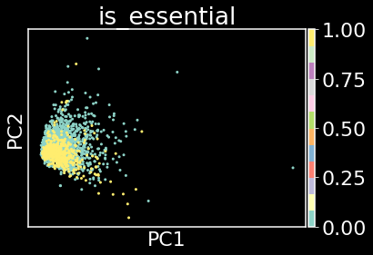
Plotting PC1 against PC2 allows us to say that the essential genes (yellow data points) and non-essential genes (green data points) are not linearly separable by their CGRs alone. In other words, CGRs may not encode information of essentiality of a gene.
This leads to the question, can we identify a nonlinear embedding that doesn’t have knowledge of essentiality?
Manifold learning
Let’s explore manifold learninig as one such approach to identify this nonlinear embedding, specifically Uniform Manifold Approximation and Projection (UMAP) will be used. I highly recommend checking out this article on the algorithmic ins and outs of UMAP, as I could not provide a better interpretation and intuition.
The general idea behind manifold learning is to, from data, learn the manifold that the data is being sampled from. It may be intuitive to most of us that if we are taking measurements from a physical or biological system, we do not expect the data points to fill all of Euclidean space, even if we are able to collect as many samples as we like. This is because every system operates under constraints e.g. concentration of biomolecules cannot approach infinity. If we can learn the data generating manifold, then we analyze how data points organize on the manifold and then make conclusions about individual cluster differences. This is what UMAP was designed to do.
In short, we first make connections between genes in ambient space or in a reduced space (for example the subspace spanned by the first $k$ PCs). In other words, we build a graph where the vertices are the genes and the edges are connections between genes and the connections represent the distance between genes. Let’s build a $k$ nearest neighbor (KNN) graph using Euclidean distance in the PC space.
sc.pp.neighbors(adata, n_neighbors=20, n_pcs=20)
sc.tl.umap(adata)
sc.pl.umap(adata,color='is_essential',cmap='Set3')
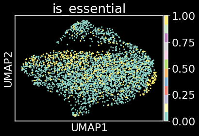
Plotting UMAP coordinate 1 against UMAP coordinate 2 allows us to say that the essential genes (yellow data points) and non-essential genes (green data points) are not separable by this unsupervised approach. It appears that we need to take a supervised approach to distinguish between essential and non-essential genes.
Metric learning
A good essential gene landscape will have essential genes far in distance from nonessential genes relative to the distance between any two essential or any two nonessential genes. Rather than defining such a distance metric, we will learn one from data. To do this, we will minimize the TripletMarginLoss of embedded CGRs. The Triplet Margin Loss encourages that dissimilar pairs of data points be distant from any similar pairs by at least a certain margin value. We will enforce this constraint not in the ambient space, but in the latent space or embedding space which will be the output of a simple fully-connect NN. As you can probably tell, there will be a lot of hyperparameters that can be optimized as well as model architectures. I won’t do any of that as this is for instructional/educational purposes only. I encourage anyone reading this to change optimizers, architectures, loss functions, etc. and find the best essential gene landscape from CGRs. In fact, you can even skip the CGRs and learn the seq2vec embedding as well!
from pytorch_metric_learning import losses, miners
import torch
import torch.nn as nn
import torch.nn.functional as F
import torch.optim as optim
from torch.utils.data import DataLoader, TensorDataset
torch.__version__
'1.8.1'
We’ll next define an MLP class for the embedding of the CGRs
class MLP(nn.Module):
    def __init__(self, input_dim, output_dim):
        super().__init__()
        self.input_fc = nn.Linear(input_dim, input_dim//2)
        self.hidden_fc = nn.Linear(input_dim//2, input_dim//4)
        self.output_fc = nn.Linear(input_dim//4, output_dim)

    def forward(self, x):

        # x = [batch size, height, width]
        batch_size = x.shape[0]
        x = x.view(batch_size, -1)
        # x = [batch size, height * width]
        h_1 = F.relu(self.input_fc(x))
        # h_1 = [batch size, 250]
        h_2 = F.relu(self.hidden_fc(h_1))
        # h_2 = [batch size, 100]
        y_pred = self.output_fc(h_2)
        # y_pred = [batch size, output dim]

        return y_pred
Define model parameters and train the model
embedding_dim = 50
model = MLP(X.shape[1], embedding_dim)
optimizer = optim.Adam(model.parameters(),weight_decay=0.0)
loss_func = losses.TripletMarginLoss()
device = torch.device('cuda' if torch.cuda.is_available() else 'cpu')
BATCH_SIZE = 32
X_tensor = torch.tensor(X)
y_tensor = torch.tensor(adata.obs.is_essential)
train_data = TensorDataset(X_tensor, y_tensor)
train_loader = DataLoader(train_data,shuffle=True,batch_size=BATCH_SIZE)
# training loop
for epoch in range(250):
    for batch_idx, (x, y) in enumerate(train_loader):
        optimizer.zero_grad()
        embeddings = model(x.float())
    #     hard_pairs = miners(embeddings, labels)
        loss = loss_func(embeddings, y)
        #     loss = loss_func(embeddings, labels, hard_pairs)
        loss.backward()
        optimizer.step()
model.eval()
MLP(
  (input_fc): Linear(in_features=256, out_features=128, bias=True)
  (hidden_fc): Linear(in_features=128, out_features=64, bias=True)
  (output_fc): Linear(in_features=64, out_features=50, bias=True)
)
model_embeddings = model(X_tensor.float())
model_embeddings = model_embeddings.detach().numpy()
edata = sc.AnnData(model_embeddings)
edata.obs = adata.obs
edata
AnnData object with n_obs × n_vars = 3309 × 50
    obs: 'organism_id', 'gene_id', 'gene', 'protein_id?', '?', 'biological process', 'biological function', 'bacteria', 'genome_ref', 'media', 'locus_tag', 'GO_id', '??', '???', 'seq', 'is_essential'
Are the embedded CGRs linearly separable?
sc.tl.pca(edata,n_comps=2)
sc.pl.pca(edata,color='is_essential',cmap='Set3')
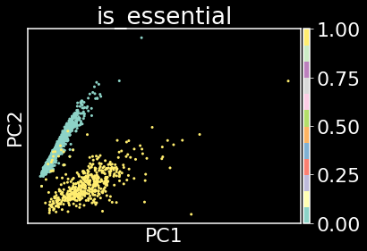
The answer is potentially.
The above plot indicates that there is signal in the CGRs that can be exploited for separability of essential and nonessential genes. However, we trained the model on all sequences and are displaying results of the embedding of the training set. To test the model, let’s make essential gene predictions for all the other bacteria in the essential gene database.
We first need a classifier that takes in the embedded CGR and outputs whether it is essential or not.
Classification in learned metric space
Given the above linear separability, let’s train a logistic regression classifier to distinguish whether a CGR belongs to an essential gene or not
from sklearn.linear_model import LogisticRegression

lr_model = LogisticRegression(random_state=0,class_weight='balanced',C=2000,solver='liblinear') \
                                .fit(edata.X, y_tensor.numpy())
Let’s make predictions for all other bacteria in the database of essential genes
acc = {}
for bacteria in anno_df.bacteria.unique():
    test_bacteria_df = anno_df.loc[anno_df.bacteria.isin([bacteria])]
    k = 4
    X_test = np.zeros((test_bacteria_df.shape[0],(2**k)*(2**k)))
    cgr = CGR_SeqAlignment()
    for ii, this_id in enumerate(test_bacteria_df.index):
        seq = test_bacteria_df.loc[this_id,'seq']
        cgr_kmers = cgr.count_kmers(seq,k)
        cgr_prob = cgr.get_frequencies(cgr_kmers,k)
        chaos_mat = cgr.chaos_game_representation(cgr_prob,k)
        chaos_mat = np.reshape(chaos_mat,(chaos_mat.shape[0]*chaos_mat.shape[1],1))
        X_test[ii] = np.squeeze(chaos_mat)
    test_bacteria_embedded = model(torch.tensor(X_test).float())
    test_bacteria_embedded = test_bacteria_embedded.detach().numpy()
    preds = lr_model.predict(test_bacteria_embedded)
    acc[bacteria] = preds.sum()/len(preds)
acc_df = pd.DataFrame(acc.items(),columns=['bacteria','accuracy']).sort_values(by='accuracy',ascending=False)
plt.figure(figsize=(2,28))
plt.barh(acc_df.bacteria,acc_df.accuracy)
plt.xlabel('accuracy')
plt.grid(True)
plt.show()
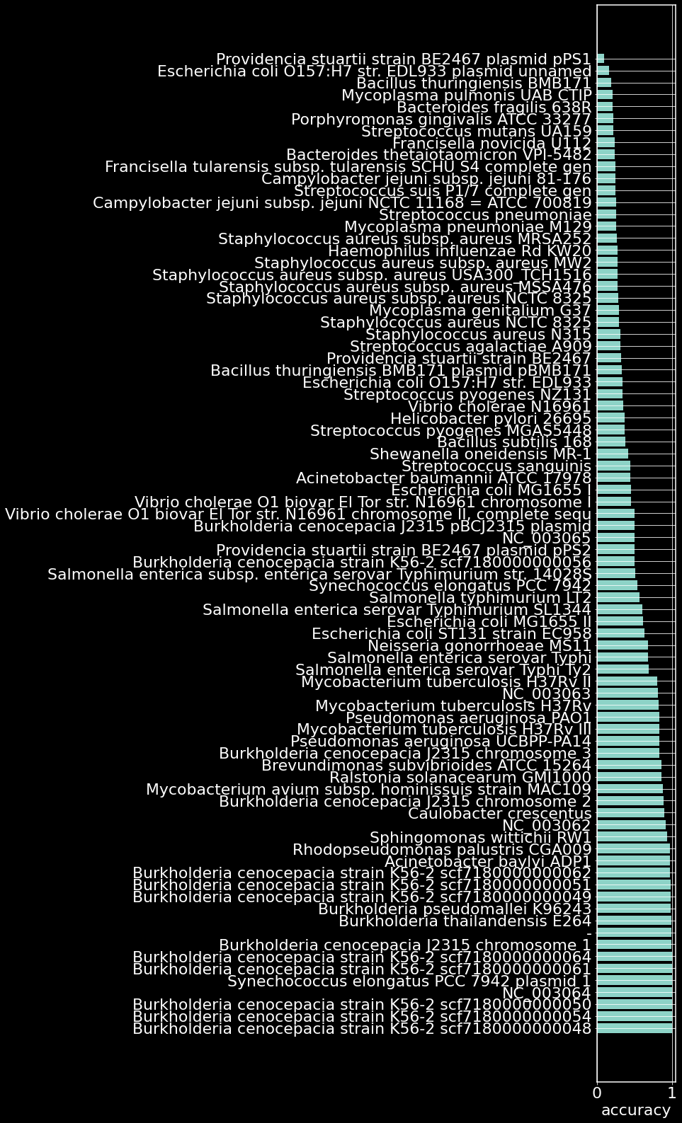
Our model of gene essentiality trained on only the ADP1 genome is able to accurately essentiallity of 30/82 organisms. Some open questions:
Does the model identify organisms with similar essentiality landscapes? How many distinct organisms should the model be trained with to ensure overall classification accuracy? We haven’t checked essential gene classfiication accuracy (as that would require scraping NCBI for the fasta files for each of the above organisms). How does this accuracy look?
Any bugs? Any questions? Feel free to let me know!